Optimal Fatigue Testing
A typical SN curve identifies the 50% fracture rate for a given level of loading. But even if the fractures were not consequential, it [...]
A typical SN curve identifies the 50% fracture rate for a given level of loading. But even if the fractures were not consequential, it [...]
We were curious about how mean stress would affect the fatigue life of the gStent-BE standardized test stent so we designed an experiment to [...]
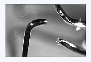
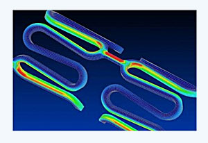
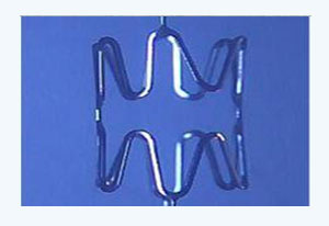
One major success of the gStent-BE as a standard test stent is the consistent fracture location during axial fatigue loading. All reported fractures occurred [...]
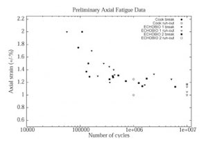
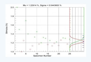
Today I presented preliminary results of our inter-laboratory fatigue study at the FDA/NHLBI/NSF Workshop. Dimensional variances were characterized for the gStent-BE and found typical [...]
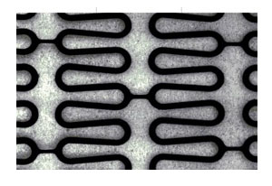
The generic balloon expandable stent, a.k.a. the gStent-BE, is laser-cut from stainless steel tubing the same as most commercially available stents. It has a [...]
The ASTM F.04.30.06 undertook an inter-laboratory study for axial fatigue testing of a generic, stainless steel balloon expandable stent. We were interested in resolving [...]